Time Series Part 1

Methodology Map

Simple Forecasting Methods

Average Method

Moving Average over a time period

Naive Method — Use the previous observation value.

Seasonal Naive — Use the observation in same season last year?

Components of a Time Series

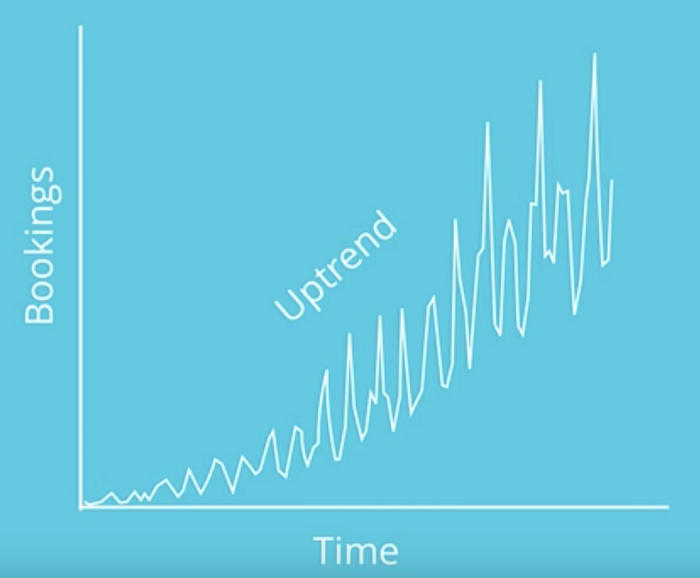
Trend: Gradual shift to higher or lower values over a long period of time.

Up trend, Down trend or Stationary

Example of an upward trend

Seasonality

Regular occurring fluctuations in the same calendar year

Cyclic pattern

Data exhibit rise and fall(Fluctuations) that are not in a fixed period

Stock market bull and bear cycles. Business cycles etc.

These are very hard to predict

Exponential Smoothing Models

ETS Time Series Forecasting

Each of these terms Error, Trend and Seasonality can be either added additively, multiplicatively or left out for smoothing method calculations.

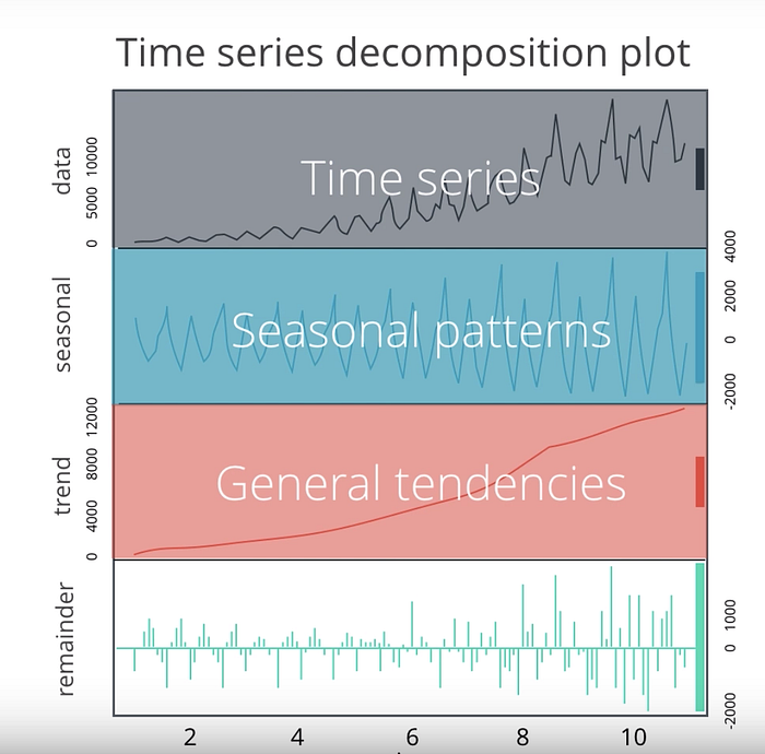
Time Series Decomposition

Seasonal Patterns with increasing seasonal values.

Upward trend. (calculated by moving average, also called deseasonalized)

Error term: Difference between Observed valued and trend line estimates. It is the remainder that is not accounted for by combining seasonality and trend.

Additive Seasonality (Sales up by 50 Units every January) show linear behavior, while multiplicative Seasonality(bookings increased 1.5 times every April)show exponential behavior.

We will explore different ETS Models that help us forecast different time series scenarios.

Simple Exponential smoothing vs Moving Average

Exponential smoothing get rids of new data faster through weights, but more sensitive to sudden large and small values.

The simple exponential smoothing method does not account for any trend or seasonal components, rather, it only uses the decreasing weights to forecast future results. This makes the method suitable only for time series without trend and seasonality.

Double exponential smoothing or Holt’s Linear Trend Method (Accounts for Trend and seasonality not

Damped Trend Methods

Holt-Winters Seasonal Method