Time Series Part 2

ARIMA

Auto-Regressive Integrated Moving Average

Seasonal and Non-Seasonal

Non-Seasonal (p,d,q)

(AR)p- no of time previous time periods used to forecast.

(I)d- No of differencing/transformations used to convert time-series to stationary.

Stationary Time-series is when Mean and Variance are constant over time. We tend to underestimate the mean and variance in a non-stationary time-series, that is why it should be converted to stationary time series.

(MA)q- lags of the error component.

Auto-Correlation — How Co-related a time-series is with it’s past values.

Auto- Correlation usually decreases with first, second differences of the time series.

AR

MA

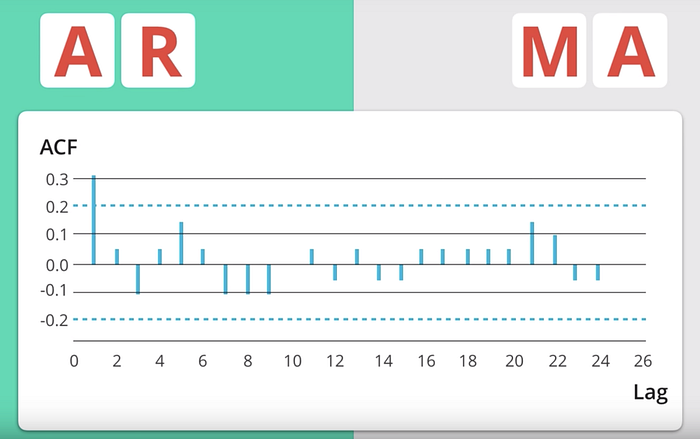
The ACF(Auto Correlation) plot helps us decide between choosing AR or MA components.

Analyzing the plot above, we have a suggestion of an AR(1) model because after we stationarized the dataset through differencing, there was positive autocorrelation at lag-1 and then the autocorrelation cuts off to zero.

If the Stationarized series has +ve Auto-Correlation at lag 1, use AR terms, if it has -ve Auto-Correlation at lag 1 at lag 1 then MA terms are better.

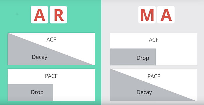
The decay/cut-off will give us hints towards what terms to use as well as spikes decaying towards 0.

When to use AR or MA terms.

Partial Auto-Correlation

Auto-Correlation between a current period and a lag period(lag2) , while controlling for the value of another lag(lag 1) is called Partial auto-correlation.

In Linear Regression terms, the more AR terms you use the more previous terms in the forecast.

ACF and PCF graphs help us determine how many AR terms we need to account for the Auto-Correlation in the series.

Auto-Regression is to account for Auto-Correlation???

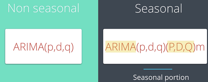
Non-Seasonal vs Seasonal ARIMA

m — no of periods in the season

(P, D, Q) — Auto-Regressive, differencing and Moving Average for the seasonal part of the ARIMA model.

Non-Seasonal differencing and Seasonal differencing are combined to staionaraize the series.

The seasonal component in seasonal ARIMA is the same as regular component except the lag is 1 season (12 months, or 365 days).

Hold out period should be at least as long as test period.

Residual Plots: Residuals should be uncorrelated.

They should have a mean close to zero and very few auto-correlation.